GWAS end-to-end
GWAS (genome-wide association study) locates genetic loci associated with a target phenotype in natural populations. The platform’s GWAS chain is now a dedicated one-page frontend form: open the GWAS workflow in the tool catalog, fill in the form once, and the full pipeline runs from QC through five-model association to annotation, plots, and report delivery — no manual tool chaining.
When to use it
- Mapping quantitative traits (plant height, yield, resistance, etc.) in natural or association panels;
- Selection-signal analysis for qualitative traits and domestication;
- Follow-up evidence gathering for candidate genes near associated loci (pairs well with database queries and the optional GO/KEGG enrichment).
Inputs and the form
| Input | Format | Notes |
|---|---|---|
| Genotype | a single VCF file, or the PLINK BED trio (.bed/.bim/.fam) | Either one; if no BED is provided, the chain automatically converts the VCF into a canonical PLINK BED |
| Phenotype table | Table (CSV/TSV) | One column of sample IDs (matching the genotype sample names) plus one or more phenotype columns; the trait column is chosen from a dropdown in the form |
The form also asks for the reference version: B73 v4 / B73 v5 / Others (other species or custom references) — this determines the annotation and enrichment background used downstream.
Pre-submission intent review: after you click submit and before the job enters the queue, the platform shows an intent confirmation that verifies the selected genotype file, phenotype file, trait column, and reference tier — mismatched files or tiers can be corrected right there, so a run never starts from the wrong inputs.
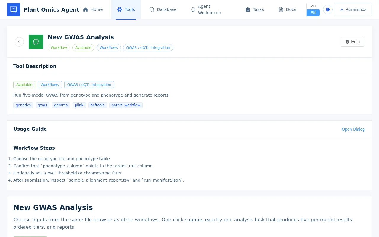
Analysis chain
QC (missingness / MAF / samples)
→ kinship matrix + PCA
→ five models in one submission (GEMMA LMM / LM + rMVP GLM / MLM / FarmCPU)
→ significance ladder, multiple tiers (strict to lenient)
→ SnpEff effect annotation (v5 by default / v3 explicit)
→ CMplot publication-grade Manhattan / QQ plots
→ self-contained HTML summary report + project delivery ZIP
→ same-version local gene annotation + optional GO/KEGG enrichment (B73v4/v5 dual backgrounds)
| Stage | What it does | What you get |
|---|---|---|
| QC | Sample/site missingness and MAF filtering | QC metrics and the site/sample counts before and after filtering |
| Population structure | Builds the kinship matrix and runs PCA | Kinship matrix and PCA plots to inform covariate choices |
| Association | Five models in one submission | Per-model association statistics tables that cross-check each other |
| Significance ladder | Multi-tier thresholds (strict to lenient) | The same results summarized at several strictness levels |
| Annotation | SnpEff effect annotation | Gene-region / synonymous / missense effect classes per locus |
| Plotting | CMplot Manhattan / QQ plots | Publication-grade figure files |
| Report & delivery | Self-contained HTML report + delivery ZIP | See “Report and delivery” below |
| Annotation & enrichment | Same-version local gene annotation + optional enrichment | Locus-adjacent gene annotations and GO/KEGG results |
Models and thresholds
The five models cover both single-locus and multi-locus families, and run in one submission:
| Model | Family | Notes |
|---|---|---|
| GEMMA LMM | single-locus linear mixed model | The mainline model, kinship-corrected for population structure |
| GEMMA LM | single-locus linear model | Without kinship, for reference |
| rMVP GLM | generalized linear model | Generalized baseline |
| rMVP MLM | mixed linear model | Kinship-corrected |
| FarmCPU | multi-locus model | Stepwise fixed-effect correction, catching what single-locus models miss |
Significance is presented as a multi-tier ladder (strict to lenient): the same association results are summarized at several strictness levels, so you can see which loci still hold at the strict tier rather than being locked into a single threshold.
Exploration exits
For a finished association run, the platform offers two exits:
- B1 read-only profile: a significance overview across the threshold tiers — a read-only summary of how many loci and which intervals pass each tier, touching no results;
- B2 bounded auto-exploration: automated tiered exploration within a preset budget cap (bounded compute and output). Exploration results carry an honest calibration status label — results that have not completed calibration are labeled “uncalibrated”, and no discovery is claimed for them.
Annotation and enrichment
- Effect annotation: SnpEff annotates associated loci (gene body / intron / synonymous / missense, etc.), using the v5 annotation library by default; choose v3 explicitly in the form when needed;
- Local gene annotation: same-version local gene annotation matching the selected reference, so locus→gene mappings agree with the reference version;
- Optional enrichment: candidate gene sets can run GO/KEGG enrichment with dual B73v4/v5 backgrounds, consistent with the upstream annotation version.
Report and delivery
When the task finishes you get two deliverables:
- Self-contained HTML summary report: a single file that opens directly in a browser, summarizing QC metrics, the five-model overview, significance-ladder tiers, and all figures;
- Project delivery ZIP: association tables, annotation tables, publication-grade figures, logs, and intermediate files in one archive — unzip and use.
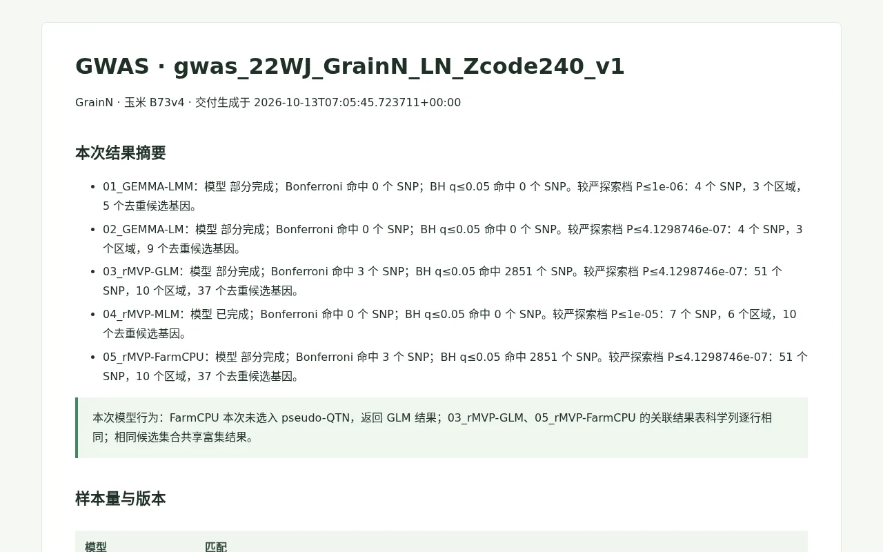
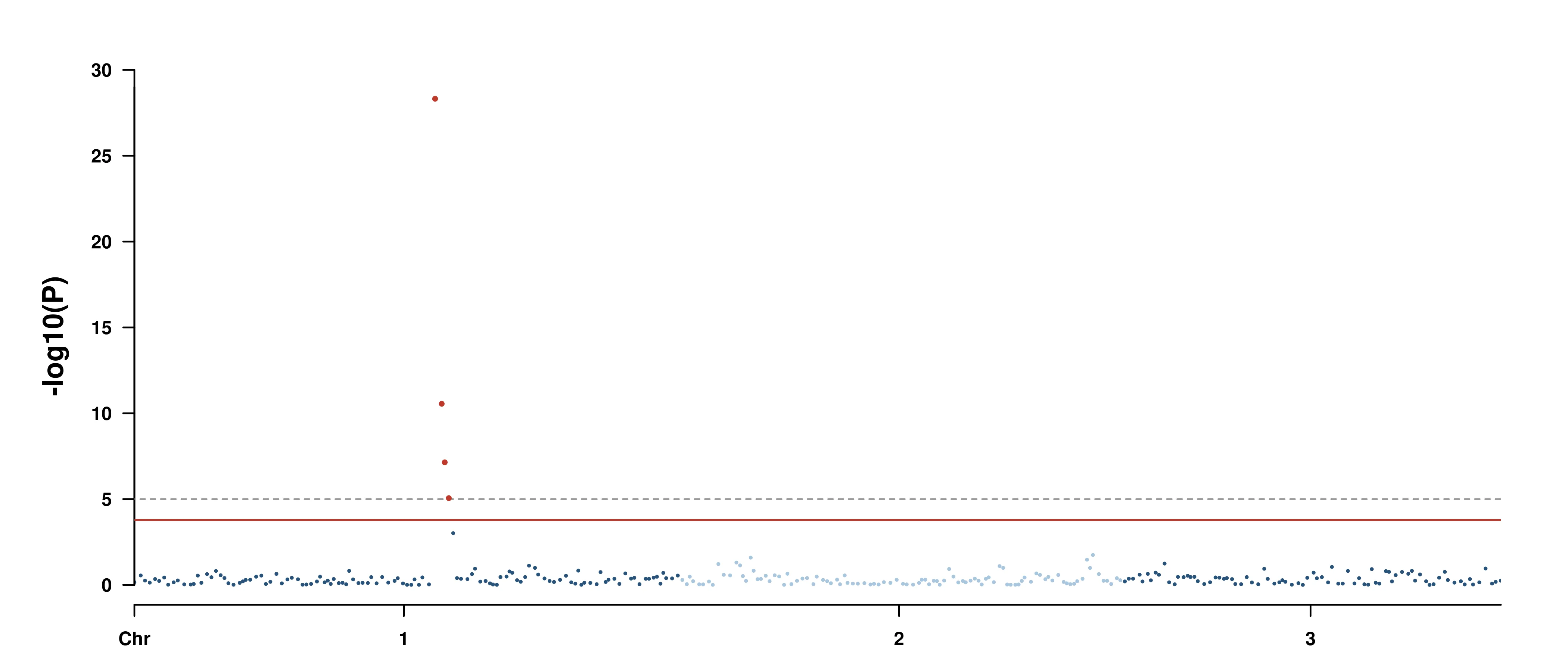
How to read the two core plots in the report:
| Plot | How to read it |
|---|---|
| QQ plot | Observed vs. expected p-values. A mid-section hugging the diagonal with an elevated tail is a healthy signal; whole-plot inflation suggests population structure wasn’t fully corrected |
| Manhattan plot | -log10(p) across each chromosome with multiple threshold lines overlaid; loci above the line even at the strict tier are the candidates to examine first |
Scale reference (real-data end-to-end validation, run-scale facts only): validated end to end twice on real data, with one full-genome rerun taking about 88 minutes; all five models completed, with 2,421,381 valid P rows per model; the delivery contained 234 files, about 458 MB.
Post-hoc exploration
Existing GWAS association results (produced here or elsewhere) can go straight into post-hoc exploration: open gwas_posthoc in the tool catalog, point it at the association result file and the exploration tiers, and explore the existing results by tier — no need to rerun the association.
Caveats
- Sample size: GWAS tests many loci, so small samples sharply reduce power; panel-level analyses generally need at least a hundred samples, and rare variants are even more demanding;
- Population structure: if your material mixes subpopulations, always use kinship + mixed models and consider adding PCA axes as covariates — otherwise false positives pile up, and whole-plot QQ inflation is the telltale sign;
- MAF threshold: set a reasonable MAF for QC given your sample size (commonly 0.05 or stricter); very low-frequency loci have little power and are prone to false positives;
- Phenotype quality: phenotypes benefit from multi-environment replicates or BLUP values; single-environment noise dilutes association signals;
- Reference consistency: the reference version used for genotyping must match downstream annotation and enrichment (don’t mix maize B73 v4 / v5, for example).